Machine Learning (ML) is a field in math and computer science that deals with creating high level abstract models to describe large and complex datasets. As a branch of Artificial Intelligence (AI), ML has existed as a discipline since at least the 1980’s, when many of its fundamental concepts and algorithms were initially theorized and published. In these early days, however, ML was primarily a conceptual field, limited in application by the relatively low computing power of the time. It is only in the last few years, with radical advances in computational and digital storage capacity, that these ideas have started to be applied at a scale large enough to see their full potential.
Many of the earliest applications of this technology dealt with very practical concerns such as web search and recommender systems, pioneered by large internet companies such as Google, Netflix, and Amazon. More recently, however, there has been growing interest in the application of these tools to art and formal design. This post will introduce our ongoing research into using a specific type of Machine Learning called deep learning or multiple layer perceptron models to create an intelligent layout of wood boards on a building facade.
Background
Although ML is a rapidly growing field, there are only three fundamental problems to which it can be applied:
- Supervised learning - the machine is presented with a small subset of data which describes a set of inputs with their desired outputs. Based on this data the machine trains a model which can be used to predict outputs on new sets of input data. If the output you are trying to predict is categorical, the application is known as classification. If it is a continuous value, it is known as a regression.
- Unsupervised learning - the machine is not given any output labels, and is asked to figure out structure in the data on its own. A typical application of unsupervised learning is clustering, and is often used for dimensionality reductions in high-dimensional datasets.
- Reinforcement learning - the machine interacts with a dynamic environment and learns through experience and real time feedback which inputs or actions will result in desirable outcomes. This type of learning is closest to how we believe humans and other organisms learn, and thus has also been studied by other fields such as behavioral psychology. One major application of this type of learning is in self-driving cars.
While many believe that unsupervised and reinforcement learning offer the greatest potential in the future, many of the early advances in ML were made based on applications of supervised learning. While this does not offer the promise of the machine learning something beyond what we already know, the ability to predict what will happen with unknown data given some data that is known has proven extremely useful in many areas such as predicting what people are trying to search for based on past search history, predicting whether a loan customer will default based on the experience of other customers, or guessing which movies people will watch based on the experience and ratings of others.
Another key application that has driven much of the technical development of supervised learning methods in recent years is in feature detection in images. Here, the computer is presented with a set of 2-d raster images which are labeled with what the images represent. Based on this ‘training set’ the computer develops a model which can be applied to new images to guess what the images contain. A key player in the development of this technologies has been Google, which is hoping to use it to allow more intelligent searches of image and video content online. We are using a similar application of supervised learning for image processing to detect the features and properties of a variable natural material - wood. To do this we will use an existing tool called TensorFlow, which has been recently released as an open-source library by Google.
The material
Our initial application of this technology is for the design of the facade of the new Architectural Lab building currently under construction on the campus of Princeton University. Given the building’s focus on environmental sustainability, we wanted to design its facade using a natural material. In several past projects we have used old scaffolding boards, so we wanted to see if we could apply it as a facade system to an entire building. Scaffolding boards are a very interesting material for several reasons. To pass inspection by OSHA, the boards need to be somewhat regular and fairly strong. However, since there is no good way to inspect them and check their performance, the boards can only be used as scaffolding for one year. After this the boards can no longer be used for their original purpose, and become a salvage material.
Using these boards in an architectural application has several advantages. Because of their demanding application, the boards are strong and come from good species of wood. Through their use outdoors for a year, they also develop a unique patina which is quite beautiful and varies from board to board. Since the board can no longer be used as scaffolding, giving them a new application is also very sustainable, since it does not require cutting down new trees or manufacturing new material. However, their prolonged exposure to the environment also creates certain difficulties, including variable cracking and warping in some of the boards. This only adds to the natural variation that any organic material such as wood has. As a proof of concept, we wanted to see if we could use advanced Machine Learning methodologies to understand something about the variations in this material, and to develop a logic that would organize it on the facade of the Architecture Lab building.
One of the main visual variations between the boards is the density and distribution of knots. Our first experiment was to see if we could train a supervised learning model to identify the location of knots in a board. We could then apply this model to each board in the facade, and use the location or density of the knots to intelligently arrange the boards on the surface. The final arrangement would be an interesting hybrid between a somewhat low-tech material with a high degree of natural variation, and an extremely high-tech algorithmic process which tries to learn from and work with this variation.
Methodology
For the proof of concept, we took a grayscale raster image of one of the boards. We then manually traced the location of the knots to create a ‘mask’ which would tell the algorithm which parts of the board contained knots, and which ones didn’t.
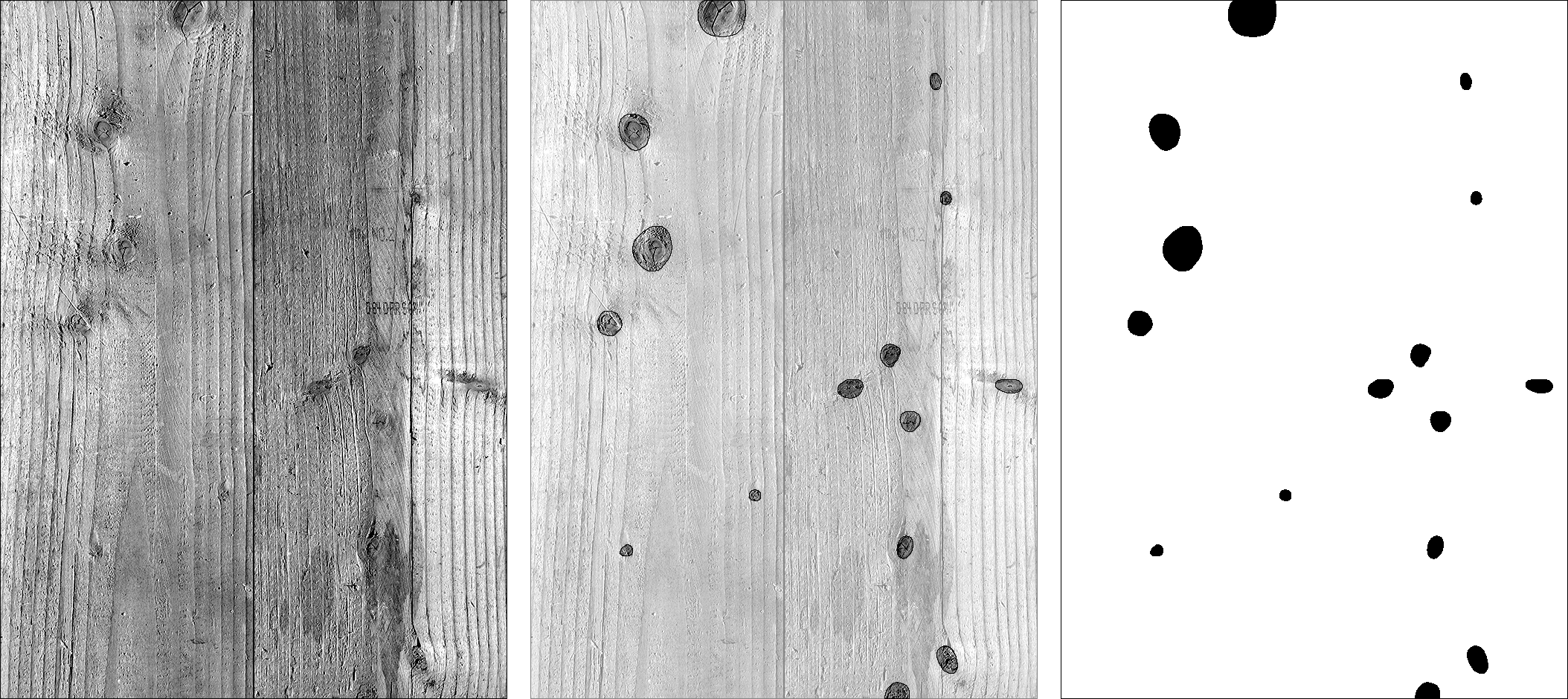
fig 1. left: original board image, middle: board image with knots overlayed, right: final mask image
The next step was to break down the image into a set of ‘samples’ which form the model’s training set. In this case, the samples are square segments of the image measuring 18 pixels on each side. Since the whole image measures 666 x 936 pixels, this resulted in 1,924 samples (37 samples across and 52 samples down). The features of each sample are the brightness values of each pixel. Since each sample measures 18 pixels on each side, this results in 18 x 18 = 324 features for each sample. These features are the ‘inputs’ or ‘independent variables’ of the model. Although it might seem impossible to learn anything about an image’s structure given just the pixel brightness values, this is actually quite common in applications of Machine Learning for image analysis.
To create the label for each sample, the corresponding mask image is broken down into the same set of samples. If the mask sample contains any black pixels, the sample is determined to contain a knot, and given the label ‘1’. If it only contains white pixels, it is given the label ‘0’. These labels are the ‘outputs’ or ‘dependent variables’ of the model. Since predicting these values is the goal of the supervised learning system, they are also commonly called the ‘target’.
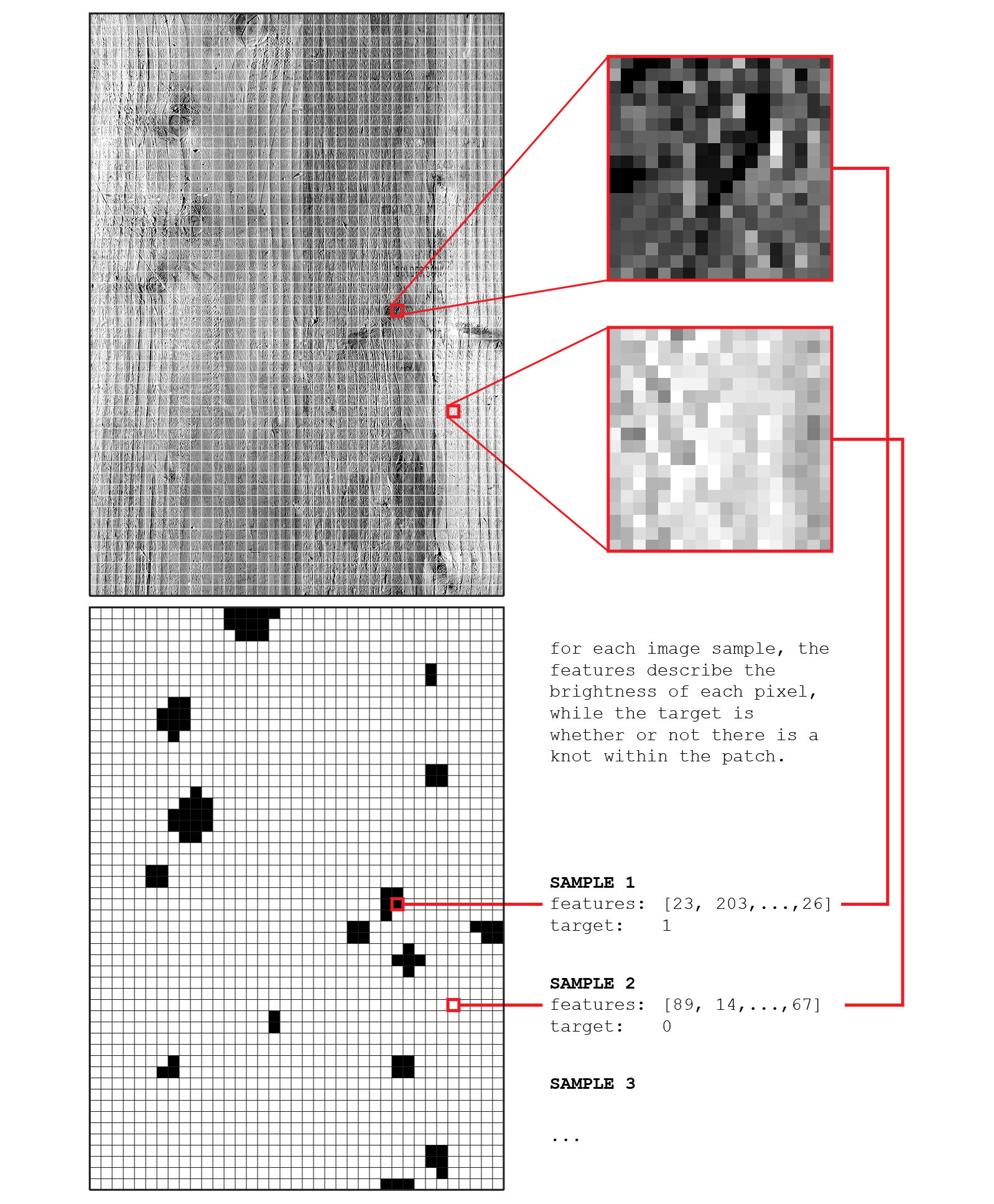
fig 2. process for deriving the training data set of the supervised learning model. Each data point is a portion of the original image. Its pixel values define the data features, and the presence of a knot defines the label or target
Once this data set is generated, it is used to train a supervised learning model in TensorFlow. For this experiment, we started with a very basic implementation of a fully-connected, single layer neural network as described in this tutorial. Following this example, we divided the dataset into three groups:
- 60% is put into a training set, which is used to train the parameters of the model
- 20% is put into a validation set, which is used to evaluate the performance of the model at each step of the training process. It is important that this data is kept separate from the training process to avoid the problem of overfitting.
- 20% is put into a test set, which is used to evaluate the final performance of the model. Keeping a separate data set for this purpose is a further measure against overfitting, and ensures that the model was in no way influenced by the data which is used to measure its accuracy. This way, the final performance number can be a good measure of the model’s ability to scale to new data sets.
Results
Based on this example, we were able to train a model which predicted the labels of the training data set with 97.5% accuracy. Fig. 3 shows the results of this model.
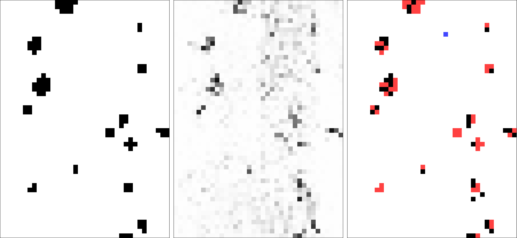
fig 3. left: desired labels for each sample, middle: predicted probability of sample having a label of ‘1’, right: samples with predicted class ‘1’ (black) with false negatives shown in red and false positives shown in blue
Although the final goal of the model is to classify each sample as either a ‘1’ or ‘0’, the model actually works through probabilities. For each sample, the model computes a probability of 0-1 for each categorical option. For example, the model might say that a given sample is 75% likely to be a ‘1’. and 25% likely to be a ‘0’ (it is common for the probabilities across all categories to equal 100%). To get the actual prediction, you would typically pick the value with the highest probability. Given this setup, it is possible to visualize the results of the prediction model according to the continuous probability of a single category (fig 3, middle), or categorically according to the most likely prediction (fig 3, right).
As you can see, though a total accuracy of 97.3% seems pretty good, in actuality the final prediction suffers from many false negatives (areas where the model predicts there is no knot, but there actually is one). This mostly likely stems from the imbalance between the two classes. Since there are so many more samples with a label of ‘0’, the model can get better performance by being very conservative with assigning the label ‘1’. For example, in this case, the model miss-classified 48 out of 82 samples with the label ‘1’. This is a success rate of only 41.5%. However, since there are relatively so few ‘1’ samples, the model is still able to get a very high performance based on correctly classifying (almost) all of the ‘0’ features [49 errors / 1,948 samples = 2.5% error rate, or 97.5% accuracy]. On the other hand, if the model was more liberal with assigning labels of ‘1’ and got all of them right while achieving the same poor accuracy for the ‘0’ sample, the overall model accuracy would be much worse [(1,766 ‘0’ samples * .575 accuracy) / 1,948 samples = 52.1% accuracy].
With this example, you can see how, with unbalanced categories, and depending on the application, it can be difficult to judge the model’s accuracy at face value. If it was crucial to locate all of the ‘1’ features as accurately as possible, this model would actually be very poor. For example, if you were trying to identify whether a tumor was cancerous, with a cancerous tumor given a label ‘1’ and a benign tumor given a label ‘0’, it would obviously be very important to accurately identify all of the ‘1’ cases, and less important to be accurate about the ‘0’ cases. In this example, false negatives are much more detrimental than false positives. With a false negative the condition might go untreated, whereas a false positive might just mean further testing is necessary.
However, in our specific case, it might actually be more interesting to look at the underlying probabilities instead of the binary prediction. Since we are developing a logic for organizing the boards based on the presence and locations of knots, it will be useful to know not only whether a knot occurs, but how confident the system is about it’s location. Dealing with the probability data directly could also solve some of the problems with false negatives. By specifying a lower threshold for when a certain probability results in a guess of ‘1’ could enable the system to find more the knots. For example, the image below uses the same probability data with a lower cutoff threshold to find more knots (you can see that this also results in many more false positives).
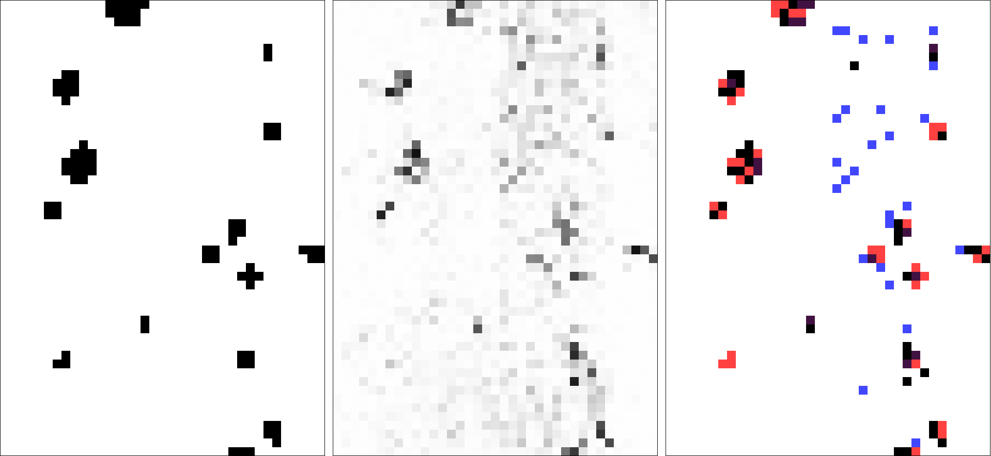
fig 4. left: desired labels for each sample, middle: predicted probability of sample having a label of ‘1’, right: samples with probability of ‘1’ higher than 25% (black) with false negatives shown in red and false positives shown in blue
Application of hidden layers
Finally, to try to get better results, we extended this model by adding one hidden layer of 512 ‘RELU’ units as described here. Hidden layers are a common way to add complexity to neural networks and allow them to model non-linear relationships in the data. In the context of image analysis, hidden layers allow the model to understand features at a variety of scales (see this article in the Economist for a high-level description). By integrating this hidden layer, we were able to achieve 98.6% accuracy, with the results visualized in fig. 5 below.
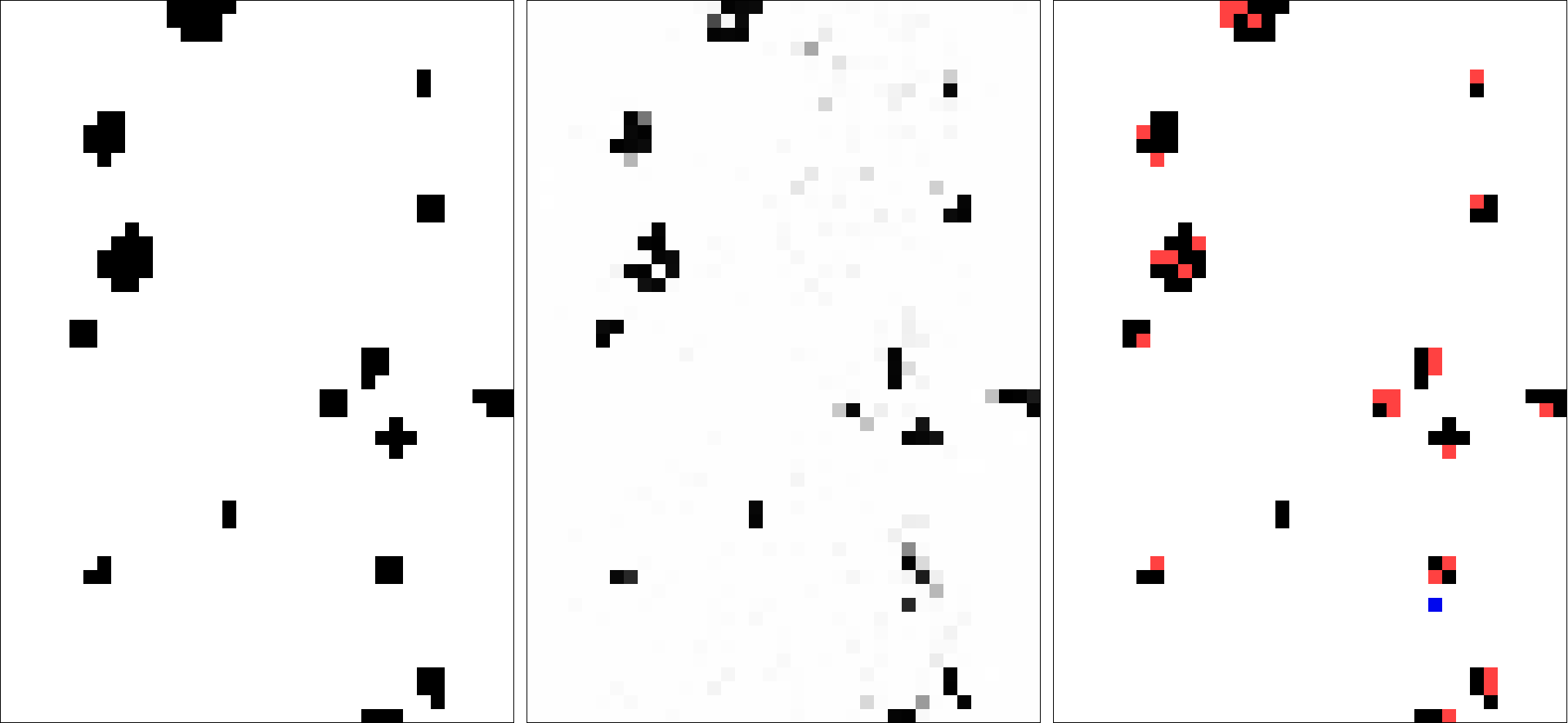
fig 5. left: desired labels for each sample, middle: predicted probability of sample having a label of ‘1’, right: samples with predicted class ‘1’ (black) with false negatives shown in red and false positives shown in blue
You can see that although a 1.1% increase in accuracy might not seem like much, in this case it translates to much better performance. The resulting prediction model achieves much better accuracy in predicting samples with a label of ‘1’, getting 54 out of 82 right (65.9% success rate compared to the previous 41.5%). More interestingly, you can see that the probability map of the label ‘1’ (seen in the middle image of fig. 5) is much tighter, with fewer gray samples. This means that the model is not only predicting the labels more accurately, but is also much more confident in its predictions.
fig 6. left: process of generating the training data, right: prediction map showing training process over several generations
Next steps
Although this is a very basic experiment, the results are very encouraging. The next steps will be to extend the model to a large training set of board images. We also want to experiment with more advanced Machine Learning models such as Convolutional neural networks to try to get even better accuracy. Finally, we are developing an organizational system that uses the knot prediction data to organize the boards intelligently on the facade of the building.