This tutorial will go over the process of setting up a workflow between a NURBS modeling software to a CFD analysis and finally to a dataset. Included are examples of usage in a general purpose exterior wind flow analysis as well as a building specific interior model. The simulation engine is Autodesk Simulation CFD 2016, which has a flexible API which allows us to build a seamless workflow into NURBS and solid’s modeling software such as Rhino, SolidWorks, Fusion, etc.
For general overview of CFD in Architecture see (following post)
Base Files
To start with, download the following base files. The default directory is C:/test/cfd, but you can change the source directory with the “init.json” initiation file. This initialization file stores information about your directory for geometry, images, results, and simulation models. Importantly, also check the installation directory of your SimCFD 2016. If it differs from the link listed in the init.json file (“C:\Program Files\Autodesk\CFD 2016\CFD.exe”), change the value for “cfd_path” to your local install.
cfd_py.zip: Python scripts and API docs (here)
base.zip: Rhino and GH geometry files with CFD setup with simple load case in 1 cubic meter wind tunnel (here)
mars_windy.zip: Rhino and GH geometry files with Toronto MaRS geometry model (here)
Geometry Creation and Automation
For the sample file, start with opening the file “solid_1m3.3dm” in Rhino and the Grasshopper script “MicroGenerative_1m3-cfd.gh.” This model will take an input from the “seed.txt” file and generate a new configuration of the five sample solids. Rhino and GH are intended to stay open during the entire process to act as a server to generate new files on demand.
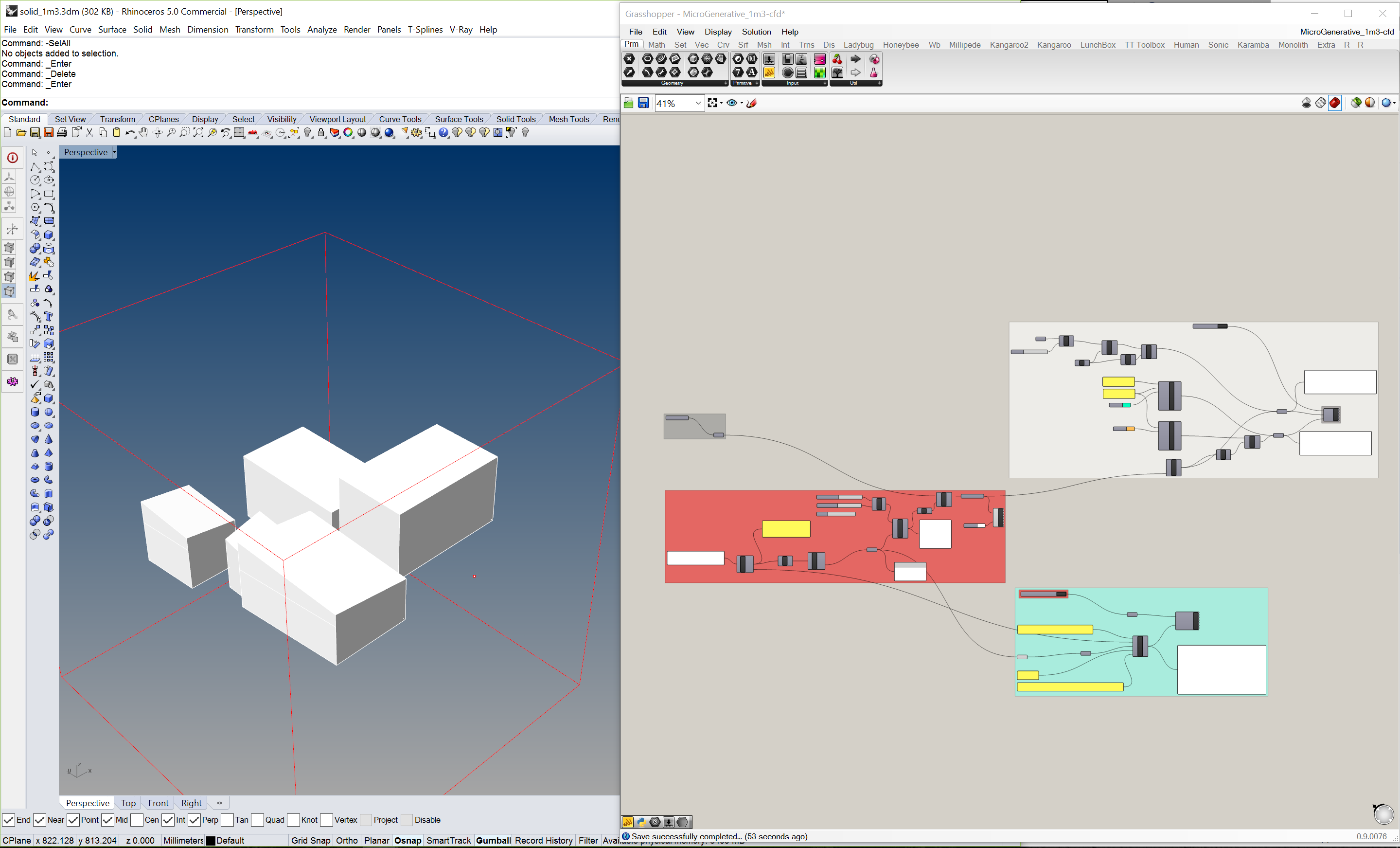
If you open “seed.txt” with notepad, change the number (any integer) and save, the Rhino model will update accordingly and output the appropriate STP solid geometry files. This update process can be automated with the included python script, “ProjectTornado.py.”” It can take arguments through the command line in the following format:
python ProjectTornado.py <mode> <CFD file> <Simulation File Directory> <Geometry File Directory> <Input Parameter>
If you supply no arguments to the python file, you can manually type in the required information through the text prompt.
Go to the directory with the python file “ProjectTornado.py” (by default this is C:\test\cfd) hold shift and right click. Select “Open Command Window Here.” Then type in the following command.
python ProjectTornado.py 1 base.cfdst C:\test\cfd\models\working\base\ C:\test\cfd\models\ 12345
This will write a new value to the input “seed.txt” file (the last value in the above command) which Grasshopper will immediately detect, update the model and output a STP file. Simulation CFD is then launched in a headless (no UI) mode and execute the API script. Through the API we can update the model, set materials, set analysis parameters, run simulation and extract results. To monitor progress in the simulation, a console log file is written out “windy_pidgy.py.log.” It is easiest to view with an auto-refreshing text editor such as Sublime Text.

The following csv file will also be written out to bridge between the python runner, the API, geometry generation, and the output dataset.
//sample input data
CFD file        ,  Project Directory                  ,  Geometry Directory             ,  Filename of New Geometry
mars_windy.cfdst,  C:\test\cfd\models\mars\mars_windy\,  C:\test\cfd\models\mars\bakery\,  123
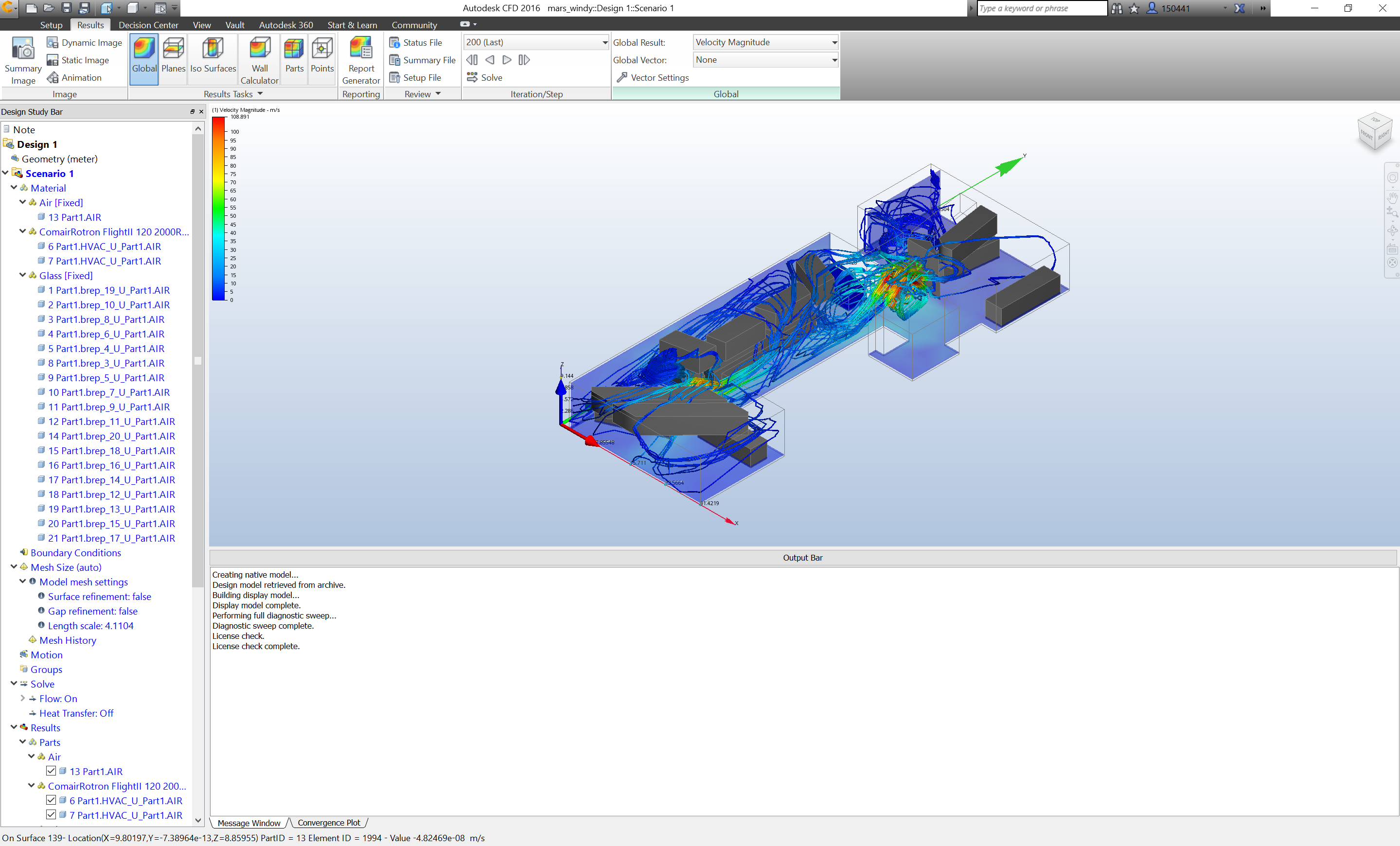
Once the simulation is finished, a screenshot will be taken (again no UI) and exported to the directory specified in the initiation file in the variable “img_path.” If you would like to change the view settings ie. colors, camera angle, result display, trace lines, etc. open the SimCFD file, go to Results, change as desired, right click on a blank spot, save view settings as view.xvs in your python directory, AND save the .cfdst file.
Finally the script adds a summary of the results to a csv dataset (“results_test.csv”). This can be opened in Excel for results analysis and plots. Results are output on an analysis grid specified by the summary plane. In the base model, this is set up as a horizontal slice the middle of the volume. This can be changed either in the “windy.py” script through the following lines. By default they are commented out in the API script, but you can uncomment and change the values for location and normal of the analysis planes.
cp1.setLocation(0.25,0.25,0.5)
cp1.setNormal(0,0,1)
More detailed results can also be taken for individual coordinates in your model. The default results output are:
‘Area’
‘Mass Flow’
‘Volume Flow’
‘Vx-Velocity’
‘Vy-Velocity’
‘Vz-Velocity’
‘Density’
‘Pressure’
‘Pressure Force’
‘Temperature’
‘Viscosity’
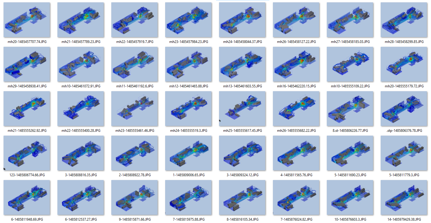
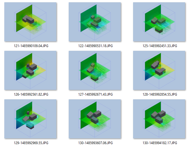
In your image directory, after a few runs, should start piling up with screencaps with a timestamp and the input value specified in the command line.
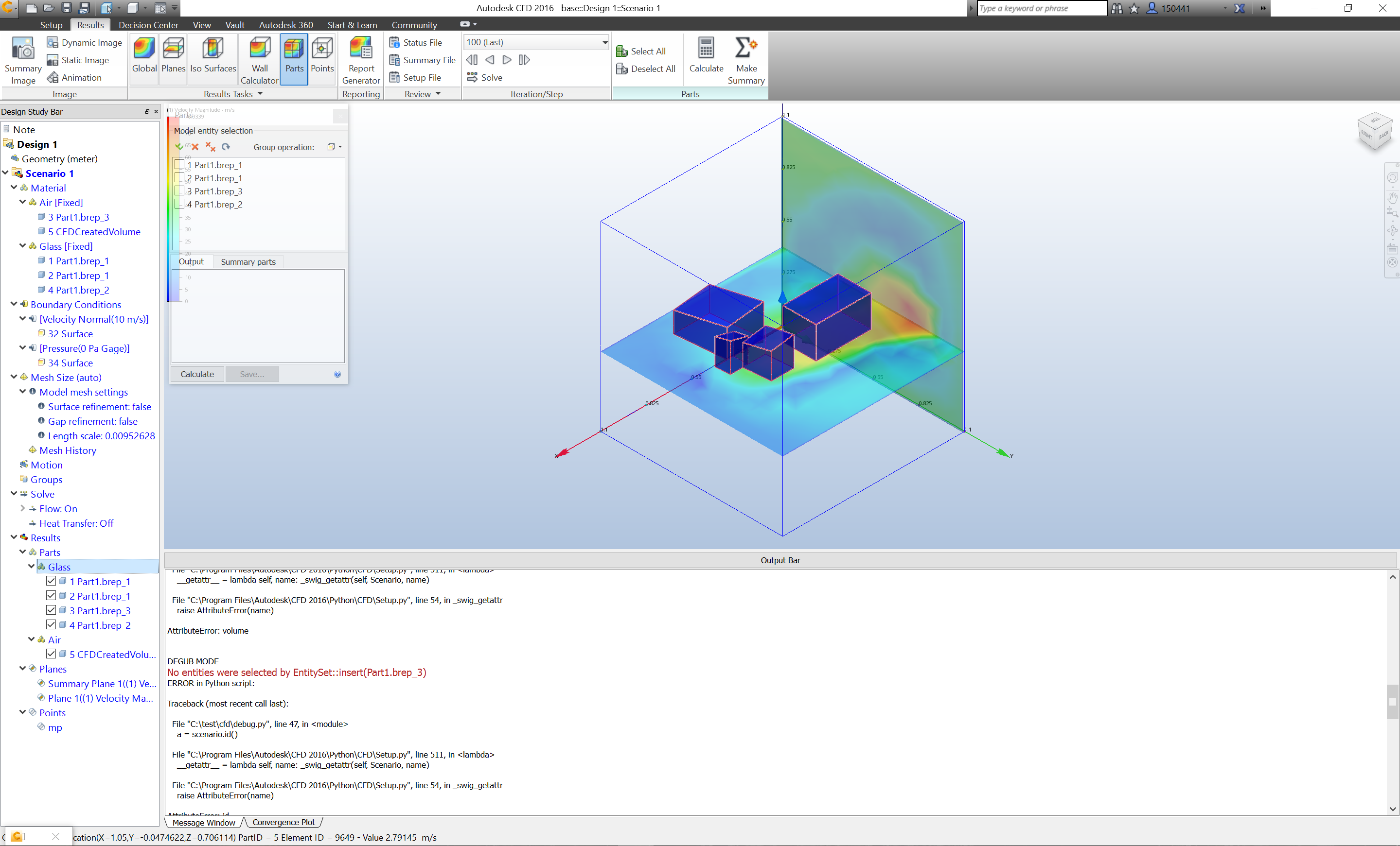
Sample 1: Wind tunnel automated models
In the second example, the Toronto MaRS office building, it requires a few additional steps to run. First, because this is an interior model, we cannot use the fixed outer bounding box as an air volume. The output from the Grasshopper script “MacroGenerative_03-cfd.gh” is an STP file with the interior air volume named “CFDCreatedVolume.” For the air supply, there are two rectangular boxes named “HVAC.” In the script “windy_pidgy.py” both objects are assigned as a high powered fan 2000RPM fan. This can be changed in the cfdst file, but to switch this in the automation, change the line scenario.applyMaterial(“your material here”) under “# Fan Material Prop.” In terms of geometry generation there are 45 different input parameters, which can be manipulated through the gene pool nodes. For simplicity, you can also use the random node with a single seed number.
Sample 2: Interior building model from Toronto MaRS project