A comprehensive generative design system for architecture would be incomplete without analysis of fluid dynamics. CFD can be used to study exterior air flows, passive ventilation, or micro climates on building envelopes. On the interior, the same simulation engine can determine HVAC air flow, interior convection currents, thermal conductivity, and the summary metric, human comfort index.
For a detailed tutorial on running the workflow see (following post)
Methodology
Through the Toronto MaRS project, The Living established a robust method for analyzing building designs for 6 comprehensive metrics including daylight, visual distraction, views, adjacency, workstyle, and buzz. We can now add fluid dynamics to our simulation toolbox with an automated link between Autodesk Simulation CFD, geometry generation, and results analysis via SimCFD’s included Python API and o2’s plugin system.
Design Implications
-
The effects of fluid dynamics are often unintuitive (at least initially) and having immediate feedback through visualizations and statictics from an advanced CFD solver running in parallel will provide a method for the designer to study and experiment with the subtle effects of form vs air flow on a building.
-
While it is common practice for a large engineering company (ie. aerospace or automotive) to comission a full scale physical prototype and wind tunnel test to verrify performance, in the architecture industry, it is extremely cost prohibitive to build a model for wind tunnel testing on most buildings except for large scale high budget projects. Computer simulations are cheaper, faster, and more acessible. They also provide the architect detailed information that are impractical for physical prototypes, such as detailed room by room interior air flow or pressure + temperature gradients.
-
Balance trade offs between air flow and other dependent metrics such as daylight, distraction, views, etc.
-
Typically air flow is handled in separate phases of a project between designer and mechanical engineers. Low resolution CFD analysis can be studied early on in the design stages using the same modeling software common in designer/architecture circles. In addition, the time consuming processes of simulation setup and post processing can be handled in an automated script.
Example Projects
CFD has been employed in at the building and city scale for decades, informing designer and mechanical engineers about ventilation performance, indoor air quality, smoke risks, and exterior wind loads. These studies typically happen in the domain of the mechanical or structural engineer after the bulk of the schematic and programming phases of the design process. Fluid dynamics have been used extensively in industries such as aerospace and automotive since the 1980’s. As simulation models have gotten better and computing power has increased, CFD has become more accessible to more industries.
Foster and Partners - Gherkin Building: Penned as “London’s first ecological tall building” this skyscraper used extensive CFD studies to inform the exterior form, the curtain wall structure, as well as flow patterns on the interior - mixing natural and mechanical ventilation.
Morphosis - SF Federal Building: One of the goals of this building was to utilize 100% natural ventilation throughout the tower. Designers even considered micro climate changes from unbuilt and hypothetical neighboring buildings as they alter city and street scale wind patterns.
The Living - HyFi: This brilliant project employed wind and structural analysis from engineers at Arup to design the supporting structure for a tower using a soft organic material which could withstand hurricane force winds.
Simulation Use Cases
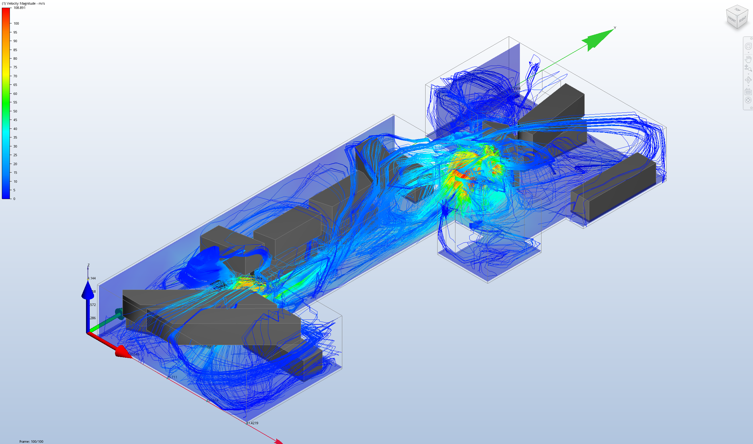
General Purpose Wind Tunnel Workflow: For models analyzing exterior air flow, we can use a general purpose wind tunnel environment. This can be done by creating a bounding box geometry with a wind velocity or fan at one end and a static pressure at the opposite end with a target geometry in the middle to analyze.
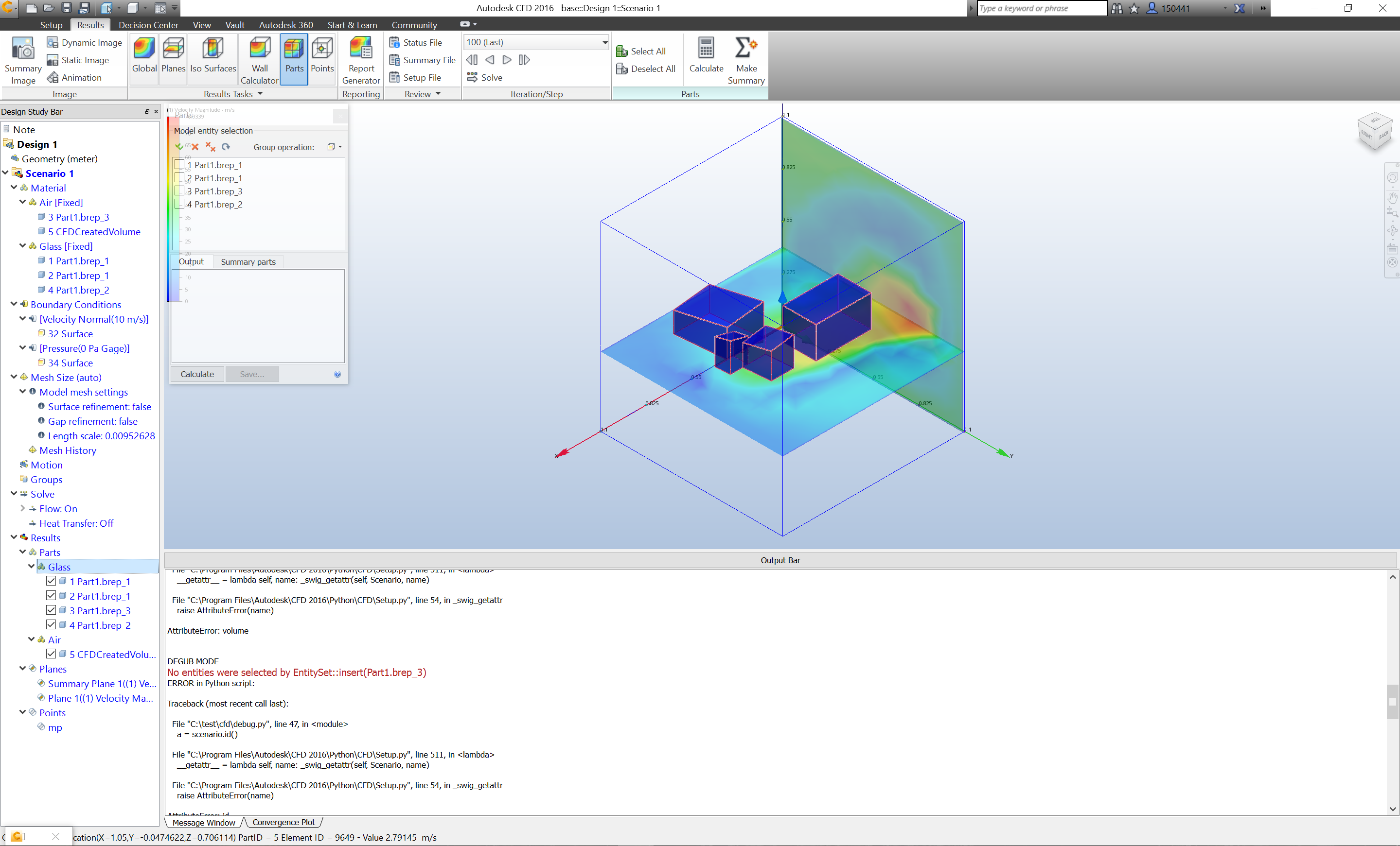
fig 1.above: Wind Tunnel setup with 1m square fixed volume and interchangeable targets (sample file here)
Building Specific Model: For more specific requirements using unique interior spaces, we need to define the air volume and materials in separate steps. The base STP file includes metadata such as object name and layer, which the SimCFD interface can identify and use to assign materials or object type such as fan, heatsink, rotating region, valve, etc. On an interior model we can also run a thermal analysis and use SimCFD’s Design Study Environment to compare the same design in multiple scenarios ie. winter vs summer.
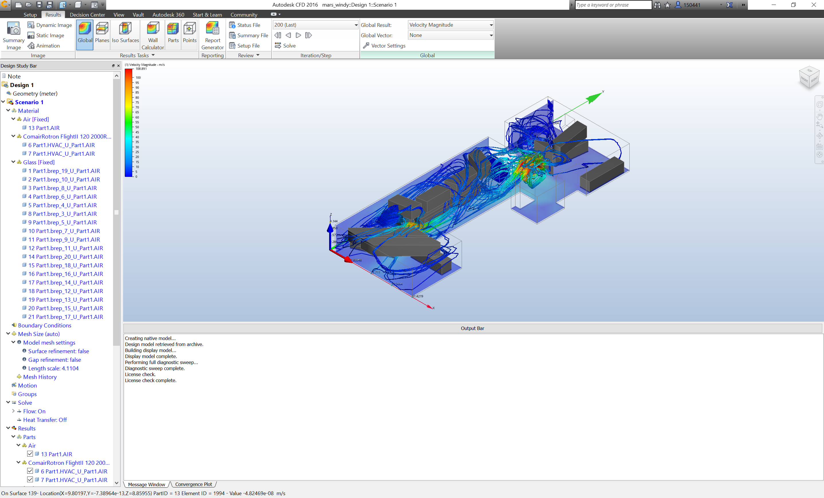
fig 2.above: Interior space analysis of Toronto MaRS building model (sample file here)
Detailed Part Analysis After an automated run, in many cases it would be necessary to zoom into greater detail on the model and plot figures along important section of the model. This is also an opportunity to re-run with simulation settings that are too time and computationally intensive to run in the larger optimization workflow ie. transient models, thermal analysis, and turbulence models requiring higher mesh resolution.
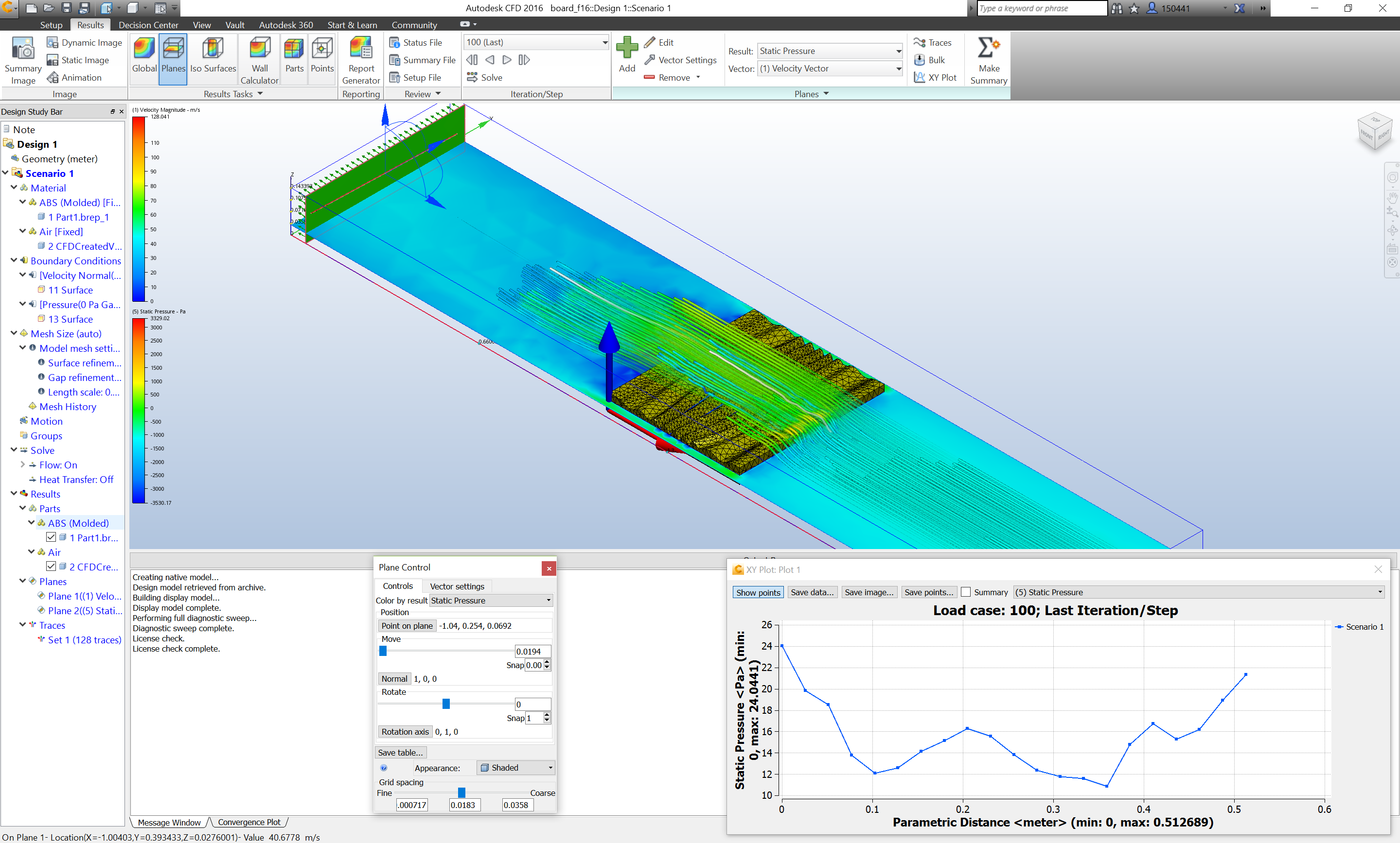
fig 3.above: Princeton sandblasted scaffold board detailed analysis (sample file here)
Geometry Creation and Automation
There are a few options for bridging geometry generation processes with SimCFD. Perhaps the simplest is through the command line interface which takes two arguments, the SimCFD install path and the base python script. It is also possible to manually create a base file, and update the geometry via the provided API tools in the UI. For our purposes, the former method is useful because both the geometry generation and analysis can be done with no UI inputs. SimCFD has a headless (no GUI) mode which can be accessed through the Windows command line and the python API.
To launch SimCFD with the script in the headless (no GUI) mode, the following function can be used to launch one or multiple designs.
# Use with Mars GD with 1 input parameter

def cfd_run_single(cfdst_path, sim_path, stp_path, seed_input):

    with open("seed.txt", "w") as f: # input file for geometry generation
        f.write( seed_input )

    with open('source.csv', "w") as f1: # input file for base sim file
        f1.write(str("{},{},{},{}".format(cfdst_path, sim_path, stp_path, seed_input) ) )

    # launch first CFD task - geometry update, materials, environment
    cmd_command = "{} -script {}".format(cfd_exe, "windy_pidgy.py")
    os.system(cmd_command)

    # launch second CFD task - visualize model with flow lines and summary plane
    cmd_command_2 = "{} -script {}".format(cfd_exe, "viz.py")
    os.system(cmd_command_2)
Simulation
Setup:
In order for python to call the SimCFD API, the following header must be added to the script. Most functions rely on the modules DesignStudy, ActiveScenario, and Results. This corresponds with the SimCFD interface for Setup, which simulation conditions are created; DSE, where designs are compared; and Results, where the detailed analysis can be reviewed.
from CFD import Setup
from CFD import DSE
from CFD import DC
from CFD import Results

study = Setup.DesignStudy.Create()
study.open(cfd_file)
scenario = study.getActiveScenario()
design = study.design( "Design 1" )

#if results exist, include following:
results = scenario.results()
Analysis:
Turbulence models:
Depending on the application, a variety of turbulence models are available. Selecting the correct model can have a dramatic effect on the results, computation time, and stability of the analysis. The Autodesk SimCFD help page (here) is a good resource on outlining the differences between each turbulence model. Our first example uses the k-epsilon model with turbulent flows while the second example uses the SST k-omega turbulence model.
k-epsilon: Default general purpose turbulence model. Stable with low memory requirements. Less accurate for models with high pressure gradients or strong curvature. (1)
SST k-omega: Ideal for external aerodynamics. Robust model with long compute times. No wall functions calculated. High levels of mesh refinement required. (2)
Scale Adaptive Simulation (SST k-omega SAS): Transient analysis ie. vortex shedding and wake structures. High levels of mesh refinement required. (3)
Detached Eddy Simulation (SST k-omega DES) High Reynolds external aerodynamics (4)
Low Re k-epsilon: Low speed turbulent flows. (5)
RNG, Eddy Viscosity, Mixing Length Other alternatives to the k-epsilon model with variations in accuracy, stability, and recommended use. (6)
Results
For the automotive industry, CFD products are the second most used software type (CAD is first). A single analysis on the front end of a car (7) can inform the designer (with given metric) on a broad range of categories:
- Front grille size and shape (volume of air moving through opening)
- Fan settings required at different speeds and throttle control (volume of air over radiator)
- Heat dissipation around engine (volume and velocity of air passing over high temp components)
- Passenger interior comfort - from the typical considerations such as ventilation to high fidelity analysis of the sound of the wind passengers can hear!
- Windshield de-icing (temperature gradient from interior/exterior)
- Brake disc cooling (volume of air passing over brakes)
- Drag coefficients of front and side profiles (force at surface)
These metrics fit into three categories which can be applied to larger scale architecture projects:
- Flow control at a specific location
- Temperature gradient between separate components
- Turbelance created by a given geometry
Results from Simulation CFD
In order to extract results from the model, we need to either create a monitor point or a summary plane. The monitor point probes the analysis results at a specific 3D point while the summary plane takes values from a 2D plane.
#Create summary plane and extract results

cp1 = Results.CutPlane.Create(results, "Plane 1") # create cut plane
cp1.setLocation(0.25,0.25,0.6) # set location of cut plane
cp1.setNormal(0,0,1) # set the orientation of cut plane

sp1 = DC.SummaryPlane.Create(study.decisionCenter(), cp1) # convert cut plane to summary plane

min, curr, max = 0.0, 0.0, 0.0
err, min, curr, max = cp1.getGridSpacingValues(min, curr, max)
DSE.UI.ShowMessage( "\tmin = %g   curr = %g   max = %g" % (min, curr, max) ) # general general summary values

summary_data = []

sp_results = DC.SummaryItemResults() # get detailed results from SP
sp1.getResults( sp_results )

for resultType, design in sp_results.iteritems():
    for designName, scenario in design.iteritems():
        for scenarioName, val in scenario.iteritems():
            resultStr = DC.SummaryPlane.ResultTypeToString(resultType)
            name = designName + "::" + scenarioName
            val = resultStr + "=" + str(val)
            val = str(val)
            DSE.UI.ShowMessage(val)
    summary_data.append(val)

summary_data = str(summary_data)[1:-1]
print("\n\n\n SUMMARY DATA: ",summary_data,"\n\n\n")
Next Steps
-
Connect with FEA Solver and broader optimization objectives to create a multiphysics environment. The types of models generated in this process lend themselves well to NASTRAN structural simulations due to their well structured solid geometry. Structural, fluid dynamics, and thermal all rely on metrics from each other (in the real [non-digital] world) and simulations should reflect this.
-
Build optimization model of building with multiple objectives derived from fluid dynamics.
-
Connect with o2 opttimization engine.
-
Develop workflow in geometry system that lends itself better to CFD and multiphysics simulations ie. level set.