There is no shortage of geometry systems for a designer. Between meshes, BREP, subdivs, and many others, all have a broad range of specialties and common uses. But the voxel has been conspicuously absent from the designer’s toolbox. Historically there have been a few good reasons for this. Voxels are very computationally expensive, and volumetric representations tend to be very blocky - even for smooth geometry. Compared to mesh representations, which have been optimized for fast ray-tracing for rendering, voxels require much more data to build comparable graphic representations. NURBS modeling has widespread appeal for its free-form surface editing and direct translation to CAD/CAM tooling. But voxels currently only have small niches in computer graphics in the form of MRI scans, Minecraft, 3D terrain representation, and pre-processing for FEA (of these options, only Minecraft can be considered a design tool).
Voxels have a number of advantages over mesh and BREP geometry, which are becoming increasingly apparent in current demands of additive manufacturing and high-resolution FEA. Voxels can provide direct representation of physical properties of solid materials and multi-material composites and as a result, a direct connection to FEA and CFD simulation. High resolution 3D printing, especially for multi-material applications and anisotropic materials, can also be much more efficiently and accurately defined as voxels.
Background
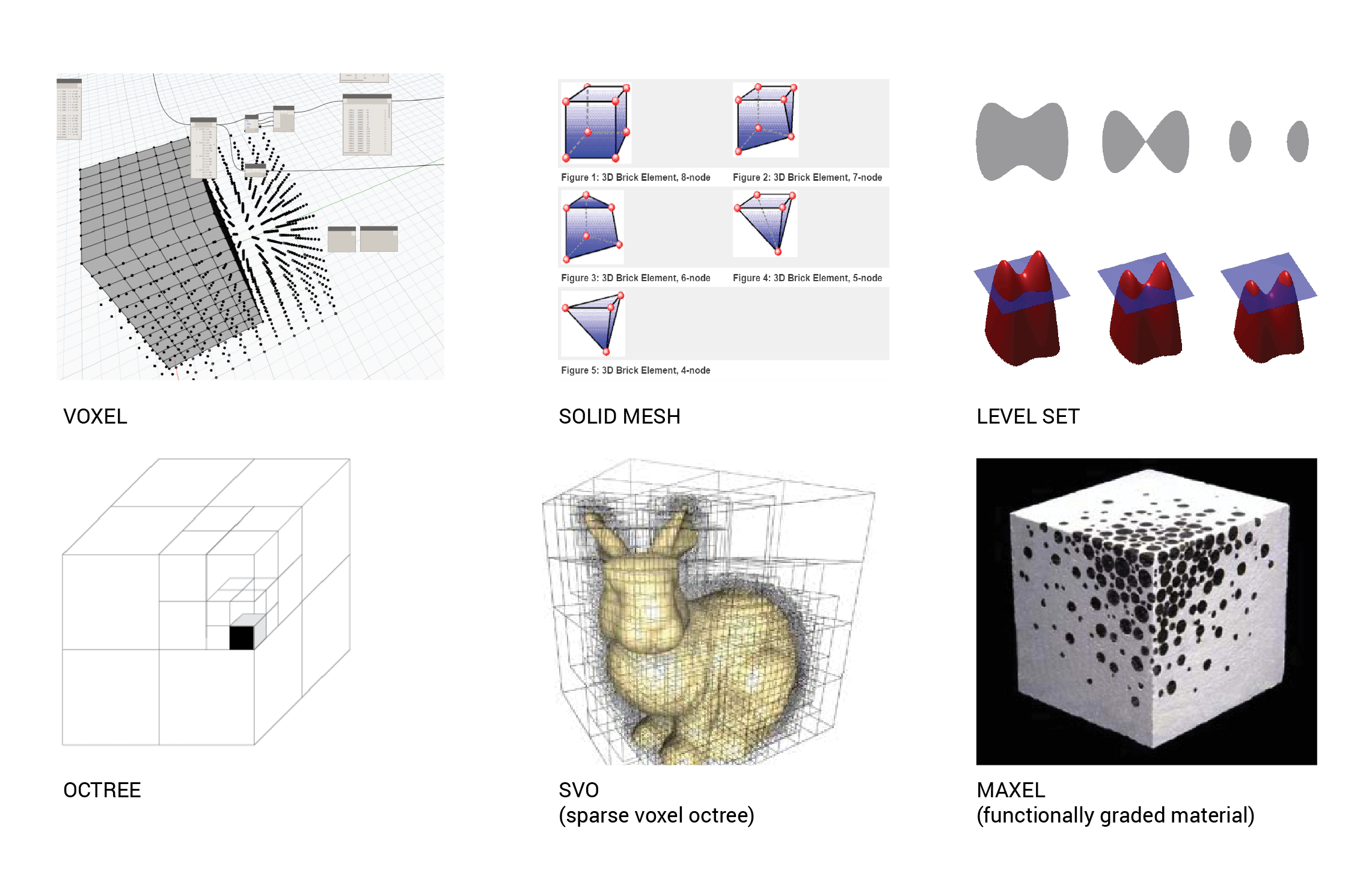
Depending on the application, there are a number of different approaches to design via volumetric geometry. Beyond the tradition voxel cube, solid meshes (which can be 8 node hexahedrons, 4 node tetrahedrons, and everything in between) are essential for FEA applications, which represent solid geometry broken down into little bricks with physical properties encoded into the edges. Octrees and SVO’s help solve one of the weakness of voxels - data intensive requirements - by optimizing and subdividing the solid into more manageable structures which can then be used in raytracing. Maxels define variable solid material properties to be used in 3D printing (especially SLA and SLS), as well as high fidelity thermal and structural applications.
Our goal is to take advantage of new generative design methodologies to operate directly on matter in 3d space. Unlike traditional parametric models, this is a less formal approach, with fewer topological assumptions. A common example is structural topological optimization in which structural forces are used to define a solid. Other potential generative systems can include agent based approaches using biological growth such as trabecular bone growth or slime mold. Recent advances in machine learning can also be applied on a 3D design space to provide truly unique and unaexpected results.
Problem: The translation between surface representations and volumetric geometry is very complicated and computationally expensive. It is impractical to represent small scale micro-lattices with surface meshes or BREPS, especially when non-uniform, anisotropic materials are modeled or simulated.
Solution: Operate directly on 3d geometry without intermediate boundary surface representation.
Methodology
We propose using the Nastran file format to directly build, control, and simulate volumetric geometry via a workflow using Dynamo, Python, and Autodesk Nastran. Dynamo is used to generate and manipulate the base voxel geometry while Python simultaneously creates the text blocks of the Nastran bulk data file. The resultant Nastran data file can then be executed through command line, with results being written and returned to Dynamo. The Living currently uses a varriant of this workflow to optimize lattice beams in Nastran and Dynamo. But we can easily expand the scope to include more complex geometry systems which better represent they physical world.
Nastran
NASTRAN has endured as the industry standard for FEA solvers in aerospace, automotive, and maritime engineering since its development in the 1970’s by NASA, and is currently being used by leading industrial engineering companies such as Airbus. It is a solver that has been validated as an efficient and highly accurate FEA analysis program with general purpose solvers being used in everything from bridges, skyscrapers, and space shuttles.
The base Nastran file is a structured dataset using fixed 8 or 16 character field bulk data entries to define model geometry and connectivity as well as material properties, constraints, and loads. Basic geometry inputs including 1d beams, 2d surface meshes, 3d volumetric geometry (tetrahedrons, prisms, pyramids, hexahedrons) and give the designer the building blocks to model almost anything one can imagine. Such models can be subjected any of the available simulation environments including structural, thermal, fluid dynamics, electrical, modal frequency response, among others.
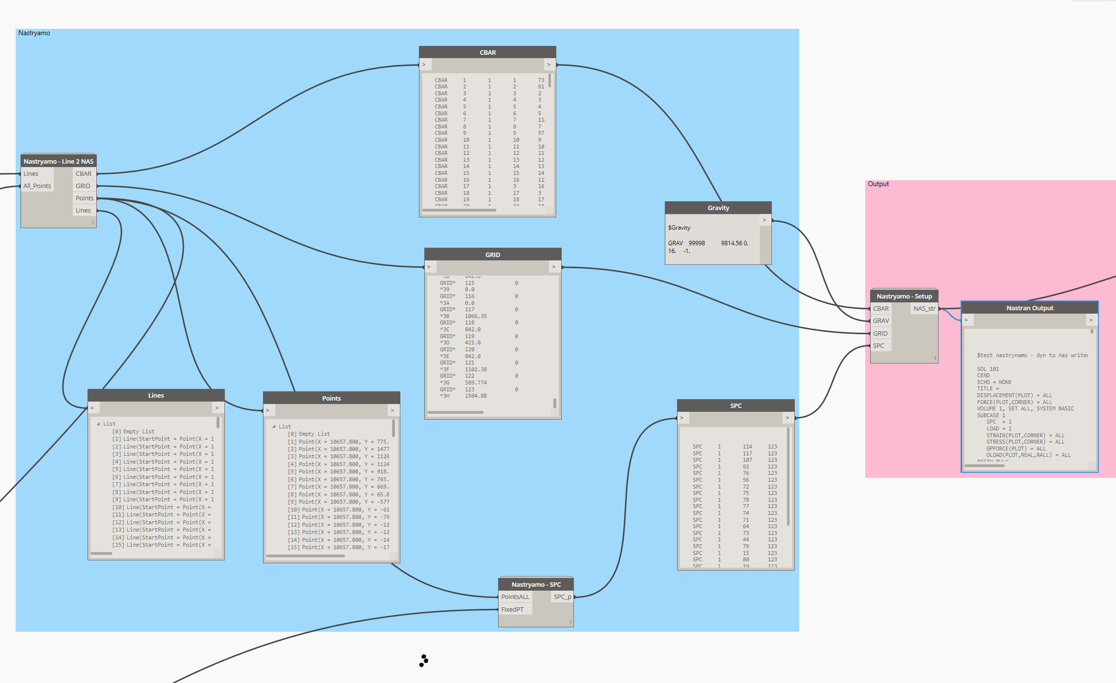
Nastrynamo Dynamo Plugin
To facilitate the creation of Nastran geometry, we have started creating a plugin for Dynamo convert dyn geometry into NASTRAN bulk data files. The plugin will aggregrate points, lines, constraints, and materials as well as run the simulation via Nastran command line inside the Dynamo Python nodes.
Geometry creation
The .nas data file is a clunky but human readable, parseable, and therefore editable file format. The base element is the grid, whose ID’s and coordinate systems are then referenced by geometry element definitions for connectivity and location. Element definitions then reference material properties. Examples of the setup can be:
Define Grid ( x,y,z, coordinate system orientation ):
GRID	ID 	CP 	X1 	X2 	X3 	CD 	PS 	SEID

GRID    1       0	9.0	2.0
Create Geometry (Voxel (Hexahedron) ):
CHEXA	EID	PID 	G1 	G2 	G3	G4 	G5 	G6
G7 	 G8

CHEXA   1       1       6       5       8       7       1       2
        3       4
Create Materials (Young’s Modulus, Shear Modulus, Poisson’s Ratio, Mass Density, Thermal Expansion Coefficient, etc):
MAT1 	MID 	E 	G 	NU 	RHO	 A 	TREF 	GE
ST 	SC 	SS 	FSM 	CS 	EC 	GC 	ALPHA0

MAT1    1       199948.         0.29    7.8547-91.17-5  0.
Define physical loads (Gravity, Pressure, Force, Fluid Flow, Temperature, etc):
GRAV    SID   CID   G    N1    N2   N3
GRAV    99998           9814.56 0.       1.     -1.

LOAD 	SID 	S 	S1 	L1 	S2 	L2 	S3 	L3
LOAD    1       1.      1.      10000   1.      10001   1.      99999
        1.      99998   0.      99994   0.      99993
One of the main limiting factors of using voxel geometry is the large number of inputs required for creating large 3D assemblies. To streamline the process for making geometry, the point grid is represented as a simple one dimensional index array and the 3D coordinate system is directly calculated from the index. For a 10x10x10 grid, index 0 is coordinate {0,0,0}, index 1 is {1,0,0}, index 2 is {2,0,0}, 10 is {0,1,0}, 108 is {8,0,1}, etc. Going from an index value to a volumetric pixel, requires finding the 8 surrounding grid points, but with this setup, it is a simple formula to define the volume, without creating 3D points or polygons. Through two simple Python definitions, we can efficiently convert from index to 3D grid and back again:
Create an 8 node hexahedron using only the index from volumetric grid. (w = grid width). Output is a Nastran CHEXA text string, formatted to the 8 character field .nas dataset.
def index2brick(ind):
    for c, i in enumerate(ind):
        c1 = int(i)
        c4 = int(i + 1)
        c2 = int(i + w )
        c3 = int(i + w + 1)
        c5 = int(i + w*w )
        c8 = int(i + w*w + 1)
        c6 = int(i + w*w + w )
        c7 = int(i + w*w + w + 1)

        voxel = "CHEXA   {:<8}1       {:<8}{:<8}{:<8}{:<8}{:<8}{:<8} \n        {:<8}{:<8}\n\n".format(i, (c5),(c6),(c7),(c8),(c1),(c2),(c3),(c4))
    return voxel
CHEXA   1       1       226     241     242     227     1       16
        17      2
Convert index of point grid into 3D point data:
def index2grid(ind):
    z = float((ind // w**2))
    y = float((ind// w)-w*z)
    x = float(ind % w)

    grid = "GRID     {:<16}{}{:<16}{:<16}*{:<6}\n*{:<7}{:<16} \n\n".format( int(b), strG1, x2 , y2 , base36encode(i-1),base36encode(i-1), z2 )
    return grid
GRID*   242             0               2.0             1.0             *7
*7      1.0
Bringing simulation results back from Nastran requires one additional step. We need to change a setting in the initialization file to output a human readable file such as ProEngineer .neu file. Autodesk Nastran can handle this via an init.ini file which is input into the command line with the geometry. The results are in a comma separated format and each row corresponds directly to the index Dynamo used to create the geometry. As a result, for visualization purposes, simulation outputs can be mapped back onto Dynamo geometry as colors or displacements. A results summary file, aptly named .rsf format, is also output with key metrics such as max displacement, stress, and mass.
Parse .rsf file for simulation results:
rsf = IN[0]

str1 = "MAXIMUM DISPLACEMENT MAGNITUDE ="
str2 = "TOTAL MASS = "
str4 = "MAXIMUM HEX ELEMENT VON MISES STRESS ="
str5 = "BAR EQV STRESS "
try:
    mass1 = rsf[rsf.find(str2, 40)+13:rsf.find(str2, 40)+25]
    mass1 = '{:40.6E}'.format(float(mass1)).strip()
    disp1 = rsf[rsf.find(str1, 60)+34:rsf.find(str1, 60)+46]
    disp1 = '{:40.6E}'.format(float(disp1)).strip()
    stress1 = rsf[rsf.find(str4, 70)+40:rsf.find(str4, 70)+53]
    stress1 = '{:40.6E}'.format(float(stress1)).strip()
    OUT = mass1, disp1, stress1
except:
    OUT = 0,0,0,0
Geometry definition
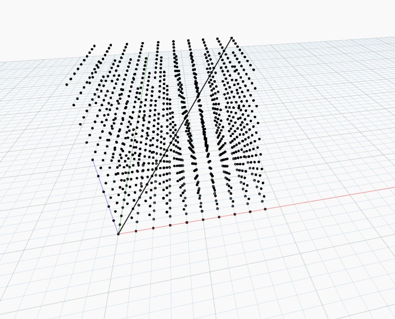
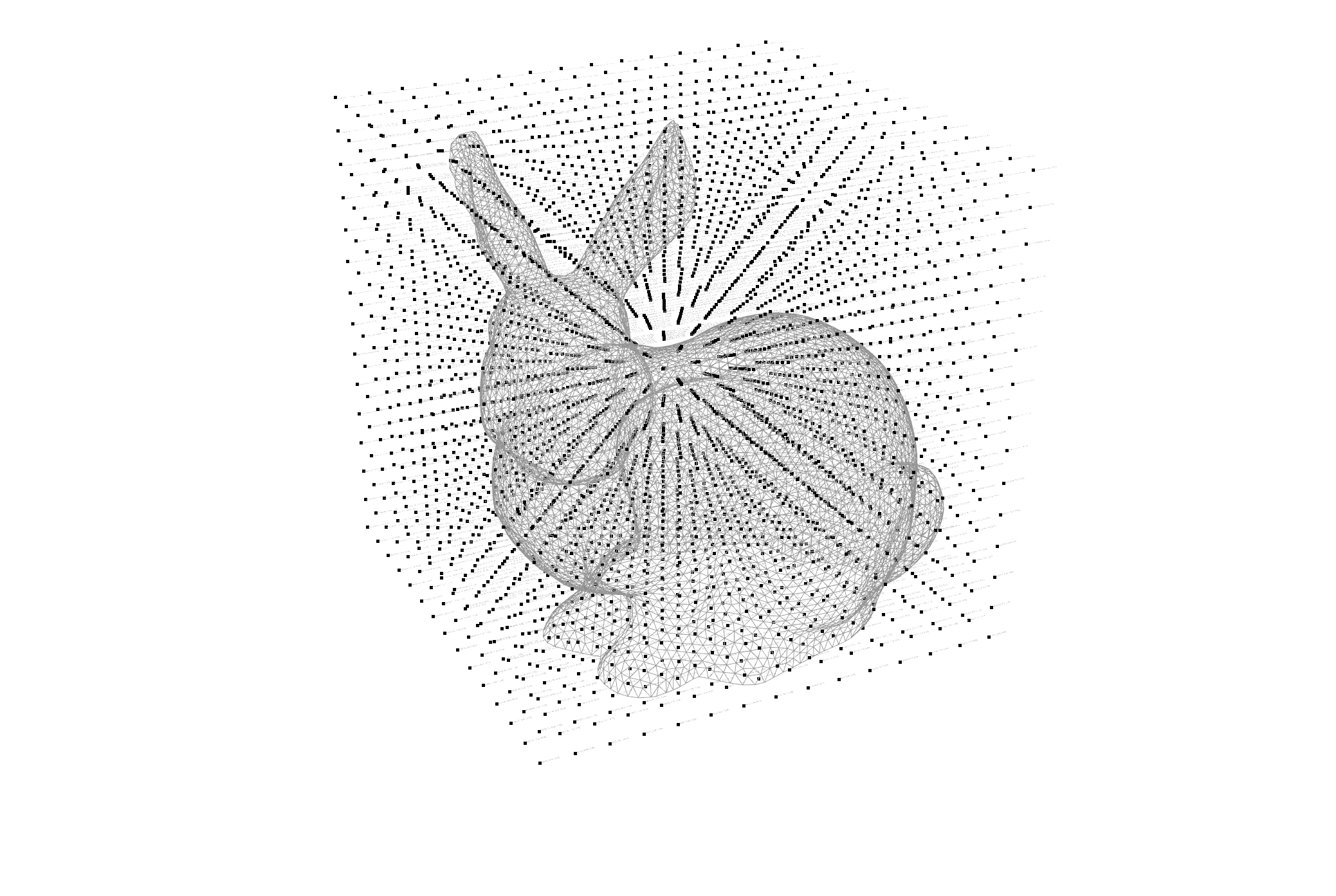
When you think of a voxel grid as a point cloud, with each point representing a {x, y, z, property1, property2, property3,…etc} dataset, you can start using formula based methods to define geometry shape, as well as physical properties such as transparency, orientation, density, mesh inclusion, etc. Operating on a point cloud can allow for solids such as spheres and cylinders to be created very efficiently with simple vector functions. Boolean functions, similarly can be used to add or subtract geometry or apply material properties.
Many of the operations for manipulating traditional 3D geometry can still be applied to voxel geometry. Inclusion tests on a voxel grid can make use of traditional surface mesh file types and create a solid voxel equivalent.
Perhaps most exciting option is defining geometry algorithmically. One tried and true method is topology optimization in which a form is defined by the structural loads through a solid. Alternative approaches include biological computation using trabecular bone growth models, agent based expansion and swarm systems, or mycelium root expansion for structural optimization. Each of these biological systems can take advantage of the state change ability of voxels and it’s ability to encode additional information. Nastran can provide the solver physical properties while Dynamo and Python can encode can each voxel with additional intelligent behaviour.
Micro-Lattices, which have been used by The Living in the design of the Airbus Bionic Partition, would also benefit from the direct Nastran voxel generation workflow. An efficient system of generating solid polygon geometry (bricks and tets) around lattice lines can dramatically streamline the processing of 3D print files and pre-processing of FEA simulations.
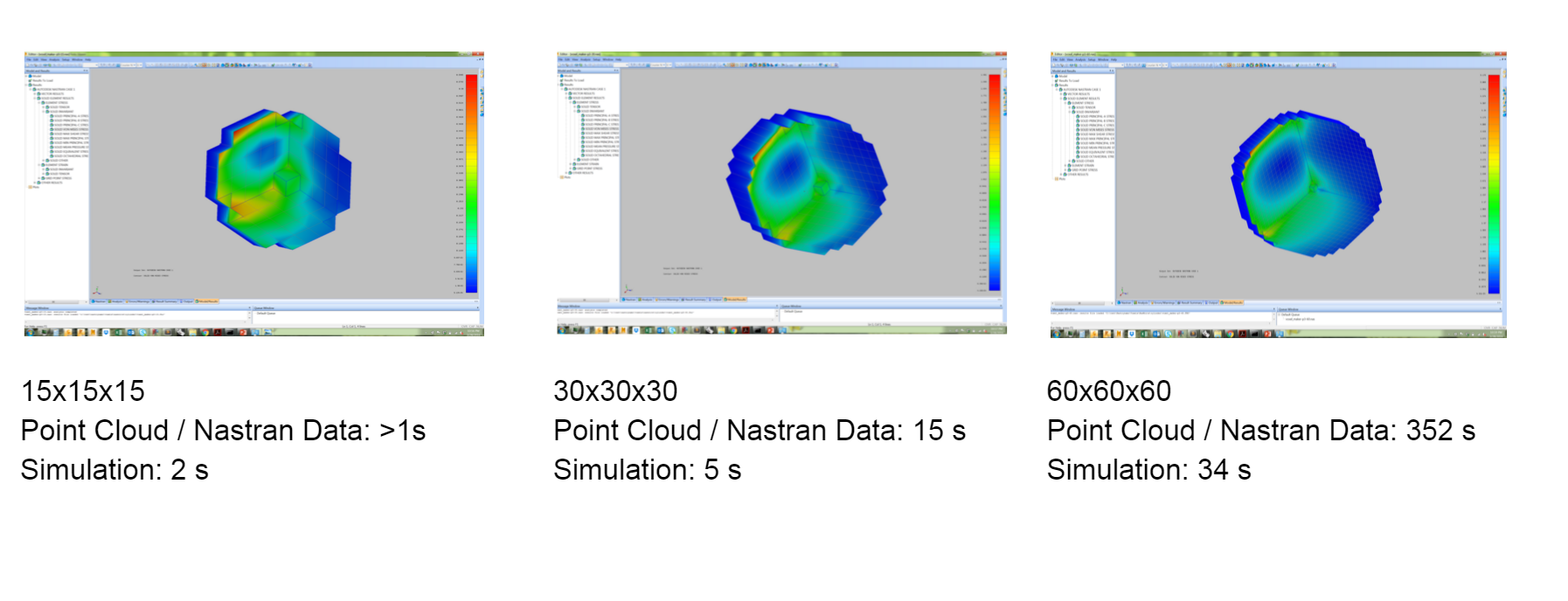
Benchmark: Cylinder vs. Bunny test
Geometry Setup: To test the voxel setup, we created a basic workspace with a square grid, a simple line to point distance function to create a cylinder, and a grid with benchmark bunny to test Nastran voxel’s ability to represent more complex geometry.
Inputs :
- 1mm grid
- Hypotenuse Line
- Cylinder radius
Outputs:
- Point Cloud { x, y, z, solid inclusion boolean, property 1, property 2,…}
- Nastran Bulk Data File
- Linear Static Analysis
Geometry Setup:
Inputs :
- 1mm grid
- Benchmark Bunny
Outputs:
- Point Cloud { x, y, z, solid inclusion boolean, property 1, property 2,…}
- Nastran Bulk Data File
- Linear Static Analysis
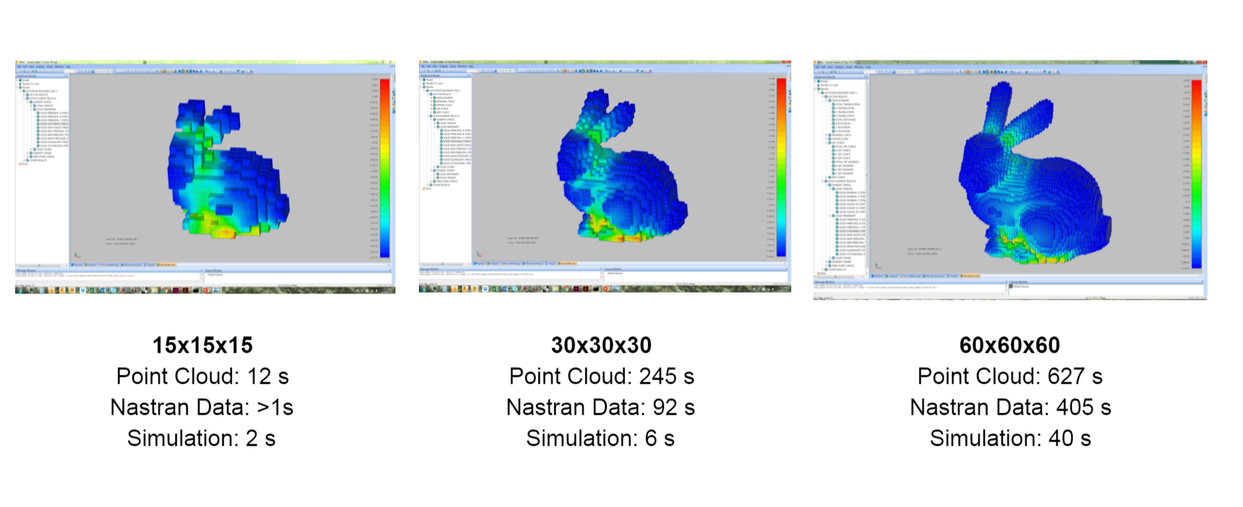
NASTRAN setup: static stress with linear material models, 16G load (in +Y direction (in direction of bunny ears) ), single point constraints below z = 0 in model, steel material properties.
Next Steps:
Surface smoothing and fine tuning: Solving the blocky and unattractive appearance of voxel assemblies is one key hurdle for voxel practicality. One option would be to perform mesh smoothing operations on the outer faces of the solid. This would not create any new geometry, and the connectivity of the Nastran data remains intact, but the locations of the grid elements will average and smoothen. Mesh refining operations that create new geometry, such as marching cubes, are also possible.
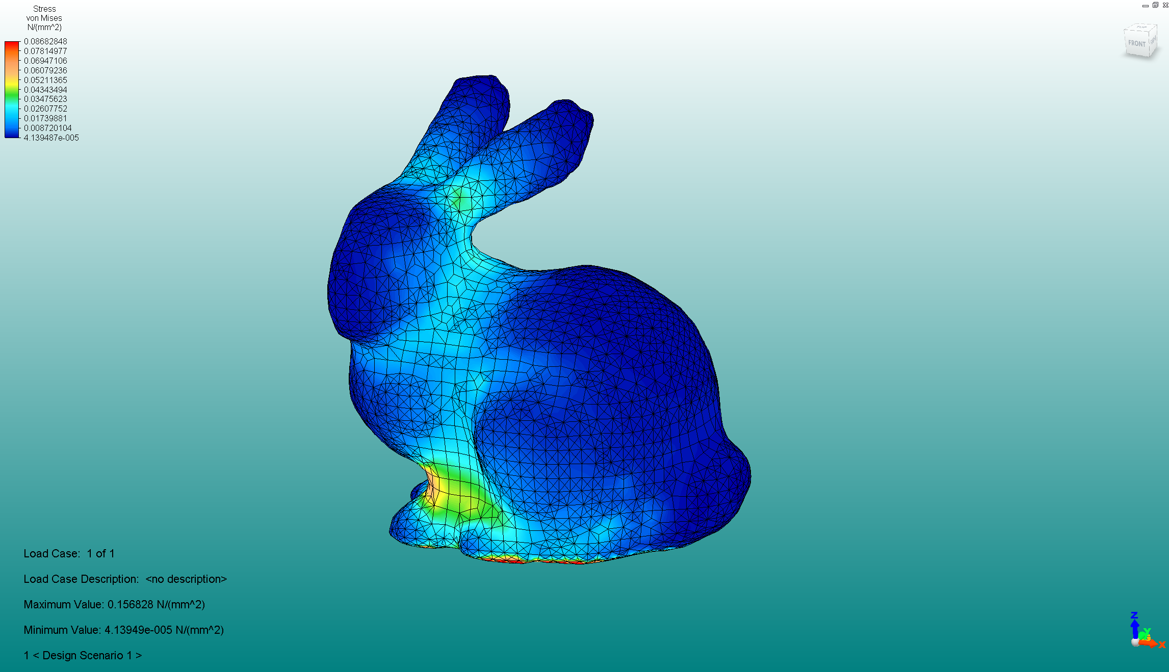 fig 1.above: 30x30x30 Voxel Bunny with Mesh Smoothing. MeshMixer, Cotan Smoothing, (scale, smoothing: 4,1): ~ 1 s. Autodesk Simulation Mechanical 2016, static stress simulation: 69 s
GPU Acceleration: Option two in making voxels less blocky is to decrease the size of the voxel to below the resolution of the 3D printer. With typical SLS and SLA printers having 0.1 - 0.01 mm resolutions, billions of voxels would be required to fill a typical build chamber. But with GPU acceleration this is not totally impractical. The nVidia CUDA Python package has shown 20x - 2,000x speed increase on benchmark tests.
Micro-Lattice representation as voxel geometry: Creating microlattices directly as solid geometry is possible using combinations of the two above methods. Computationally this would function the same as the cylinder test, with many more line calculations, as well as assemblies of mixed solid polygon voxels (tets, bricks, etc.). This would drastically decrease the pre-processing time for 3D printing and simulation.
Formula based representation of geometry: Examples in biological computation via bone growth, slime mold, or mycelium growth can operate on a voxel agent based system much more efficiently than a traditional BREP model. The voxel dataset would very easily be able to take advantage of multi-objective optimization, simulated annealing, or machine learning (ie. Tensor Flow).
Level Set Method: Volumetric geometry lends itself well to level set